How-to use Blender's geometry nodes for visualizing CMB
In this note I’m going to introduce Blender’s power to scientists, mainly cosmologists. Blender is an open-source cross-platform 3D content creation software and supports the entire 3D pipeline (see Blender’s about for more information).
We will see how to visualize CMB maps (see visualization nodes) and how we can deal with CMB maps like meshes and benefit from the parallel computation for SIMD tasks. I will show you how to import your data into Blender and work with it step by step. The methods explained here are for local computers but could be applied elsewhere (e.g. Google Colab). Each step could be a separate post but the order could be problematic in case of separation.
Creating HEALPix mesh
First, we need to create a 3d mesh out of healpix data. There are several ways to do it but the easiest way is to use healpy package.
Since at the moment, healpy is only available on Linux & mac, windows users can use wsl(windows subsystem for Linux) that allows them to run Linux terminals in Windows environment.
In the following, we will create a handmade OBJ file that can be imported to any 3d DCC. Now, in this section, we will use system’s python to create our mesh, not Blender’s, since Blender uses its own internal python, which is a separate one (Insha’allah I will write a post on how to install external modules on Blender’s python, but even if we install healpy on Blender’s python it is not still useable in windows).
First, we create a function to generate texts to make the OBJ file.
1
2
3
4
5
6
7
8
9
import numpy as np
import healpy as hp

def generate_obj_txt(element_arr, str_key):
    txt = ""
    space, next_line = " ", "\n"
    for elem in element_arr:
        txt += str_key + "".join(space + str(component) for component in elem) + next_line
    return txt
The above function creates simple texts like this:
1
2
3
4
5
v 0.0 1.0 -0.0
v 0.0 1.0 1.0
f 1 2 3 4
f 5 6 7 8
...
That defines vertex coordinates and specific indices that make a face(forget about additional data, edges, skinning data, etc., in this tutorial since we don’t need those).
Then we store pixels’ corners(boundaries) in a well-sorted way like below:
1
2
3
4
5
6
7
8
9
10
nside = 64
npix = 12 * nside ** 2
v_coords = np.zeros((npix * 4, 3)) # 4 corners for each pixel and 3 coords for each corner

for i in range(npix):
    pbounds = hp.boundaries(nside = nside, pix = i, step = 1, nest = False) # we use ring indexing
    v_coords[4 * i : 4 * (i + 1)] = np.transpose(pbounds)

v_indices = np.arange(len(v_coords)) + 1
faces = v_indices.reshape((npix, 4))
One can optionally merge duplicate vertices here by utilizing merging algorithms, but it is much easier and faster to do this process inside Blender.
Now it’s time to write the OBJ file using the above arrays of vertices and faces. Note that we have to change coordinates from (right-handed)xyz to (left-handed)xzy (y_lh = z , z_lh = -y) since it is the most usually used case for OBJ file importers:
1
2
3
4
5
6
7
8
# mesh creation
f3dname = "healpix_sphere.obj"
with open(f3dname,'w') as f3d:
    # before saving, change coords
    v_coords[:, 1], v_coords[:, 2] = np.copy(v_coords[:, 2]), -np.copy(v_coords[:, 1])
    ftxt = generate_obj_txt(v_coords, "v")
    ftxt += generate_obj_txt(faces, "f")
    f3d.write(ftxt)
For high-resolution maps(nside>1024), mesh creation is not a good approach for processing because only the mesh takes an enormous amount of memory and needs a high-end graphics card to manage. Although Blender can handle a 50M polygons mesh with a high-end graphics card, it’s not an optimized way to process data.
For high nside values (>256), it is recommended to create the mesh part-by-part; that means dividing the npix array into several sections and making a mesh for each part (you can merge all these parts in Blender). It may take up to an hour to generate a nside=2048 mesh, but it can also become heavy(about 12 GB, while with vertices merged, it would be ~2.5GB at most). So divide it and merge it part by part. We can write a script to do all that.
I would like to say thanks to Andrea Zonca, who helped me with finding the boundaries of pixels.
Importing the mesh into Blender (Intro to Geometry Nodes)
This section is for beginners in Geometry Nodes. If you already know about that, skip this part.
By opening Blender you’ll see the default objects. Click on the 3dView and press A to select them all, and press X and Enter to confirm deletion.
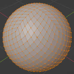
Now click on File > import > Wavefront(.obj) and head to the directory of the OBJ file you created and import it. The image below shows a HEALPix mesh with nside = 8:
As explained, the file contains many redundant vertices since neighboring pixels have duplicate vertices. To this end, we could use several different tools, but for getting familiar with Blender’s Geometry Nodes(from now on geo-nodes), we use this tool to merge those redundant vertices.
At the top bar in the far right, find the Geometry Nodes tab and click it.

If you don’t find the Geometry Nodes tab, hover your cursor on the top bar and hold MMB to pan the bar to the left to find Geometry Nodes. It is worth noting that anywhere in Blender(in 3dView, panels, etc.), MMB is used for panning, Ctrl+MMB for zooming and Ctrl+Space for maximizing view.
Now select the HEALPix sphere you imported, and click on the “+ New” button on top of the geo-nodes panel. Now you will see an input mesh and an output that are the same at the moment:

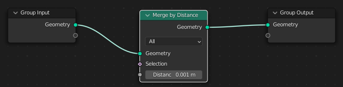
Now we want to add a node to merge duplicate vertices. Press Shift+A to open add-pannel.
Shift+A everywhere opens add menu.
At the top click on search and search merge to find Merge By Distance and press Enter. Now move it to the middle of the process and click to place it like this:
On the far right you will find Properties panel. Click on the modifier’s dropdown button and select apply.

Now you have merged all redundant vertices. Save the file somewhere for later use.
Importing map data and setting mesh attributes
In this section we are going to extract data from CMB maps and import them as face data of the mesh. First you have to extract data from e.g. Planck maps. To do this, first download one of the provided maps e.g. Commander.
Now in system’s python, read Plack map and extract its temperature, stokes_q and stokes_u data:
1
2
3
4
5
6
7
8
9
10
11
12
13
14
15
# Extracting data from .fits files
import numpy as np
import healpy as hp

nside = 64
fpath = "E:/Your/Path/" # change it for your own case
fpath += "COM_CMB_IQU-commander_2048_R3.00_full.fits"

_fields = (5, 6, 7) # inpainted fields
_names = ("temp", "stokes_q", "stokes_u")
for name, field in zip(_names, _fields):
    map = hp.read_map(fpath, field = field, nest=False)
    map = hp.ud_grade(map, nside_out=nside, order_in='RING')
    map *= 10**6
    np.savetxt("./" + name + ".txt", map) # format doesn't matter that much
Having data extracted, open Blender > stored mesh file, pan the top bar and select Scripting. In the Text Editor create a new script and enter the bellow code into it:
1
2
3
4
5
6
7
8
9
10
11
12
13
14
# Assigning attributes to mesh
import numpy as np
import bpy

path = "E:/Your/Path/To/" # change it for your own case

obj_attr = bpy.context.object.data.attributes # active object's attributes

_names = ("temp", "stokes_q", "stokes_u")
_attributes = [np.loadtxt(path + name +".txt") for name in _names]

for name, attr in zip(_names, _attributes):
    obj_attr.new(name=name, type='FLOAT', domain='FACE')
    obj_attr[name].data.foreach_set('value', attr)
The above code assigns your each pixel’s data into its analogous face in the created mesh. Assigning attributes to the mesh lets you use the power of geo-nodes in parallel computations and also visualization(in realtime!).
Visualizing assigned attributes
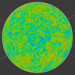
In this section we want to achieve a visualization mechanism. The result is like the image bellow:
Visualization nodes
Get back to the Geometry Nodes tab and create a new one. Create a geo-nodes graph like the one below(I will explain what all these do):
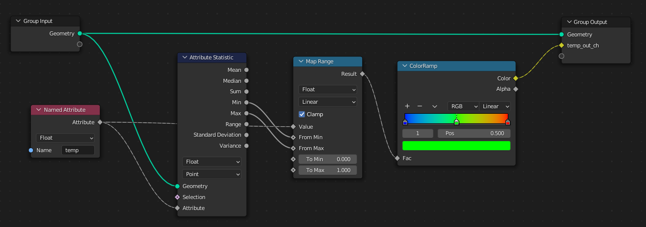
We proceed from left to right. First, the Named Attributes nodes take the data values we assigned to mesh(in the previous section) and make them visible for geo-nodes. The Attributes Statistics node reads these values and gives the outputs shown in the image (Note that it takes the Geometry wire to know which mesh we are looking for). Then we should map the minimum & maximum values of the temp attribute into the range (0, 1) by the Map Range node. The ColorRamp node maps these values to a set of color data(attributes) that is read in the materials as we will see.
To create this color ramp, click the ‘+’ button to create a new tick and enter 0.5 for its position. Then change the color of the first tick to RGB = (0,0,1), the middle one to RGB = (0,1,0), and the last tick to RGB = (1,0,0). This gives a similar gradient to the jet coloring.
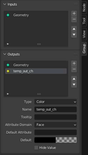
Connect the output of the color ramp to the free output socket. Press the N key to open the right panel, go to the Group tab, and rename the output to what you want e.g. temp_out_ch. Note that the type of this output is color.
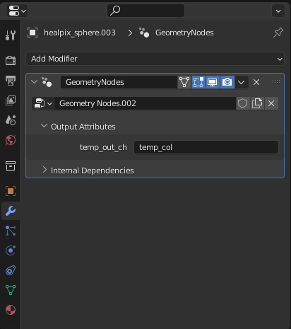
Now in the Properties > Modifier (the far right panel) put a name for the attribute that this output creates e.g. temp_col.
Material
Having the object selected, go to Properties > Materialand click the + New button to create a new material. Change the surface material type to Emission.
Then, by clicking the circle button near the color property, change the color type to Attribute. In the Name field, type temp_col(or whatever you named the attribute).

Now, in the 3dView, hold the Z key, and in the pop-up menu select Material Preview and you have to see the CMB sphere.