Lab · live demo

Spherical Harmonics

The real or imaginary part of any spherical harmonic up to degree 512, painted on a HEALPix sphere. Pick l and m, and view it from outside or as a Mollweide map.

A spherical harmonic on a sphere, in jet colours from blue (negative) to red (positive), with a Tools menu at the upper left and a menu for l and m at the foot

What it is

Spherical harmonics are the natural waves on a sphere. The degree $\ell$ counts the nodal lines across the sphere (the more of them, the finer the pattern) and the order $m$ , from $-\ell$ to $\ell$ , says how many of those lines are meridians. In the jet colours, blue is negative, red is positive and green-yellow is about zero. The colour range is set by the largest value of the chosen harmonic, so its pattern is always easy to read.

01 Why they matter

Any smooth function on a sphere can be written as a sum of spherical harmonics, as a function on a line is a sum of sines and cosines. The CMB temperature map is expanded this way, and the strength at each degree $\ell$ , its angular power spectrum, is the main thing cosmology reads from it.

The same functions give the shapes of atomic orbitals, the vibration modes of a planet, the gravity and magnetic fields of the Earth, and the lighting of a scene in computer graphics.

02 How it is built

Step 1

The sphere is built

A small Nside=16 HEALPix mesh (3,072 quads, under 1 MB) is loaded, and a web worker splits every pixel into children until the sphere has Nside=256 (786,432 pixels), or 128 on phones and tablets. Each pixel keeps its RING index.

Step 2

Each pixel is evaluated once, at its centre

A first pass draws the harmonic into a texture with one texel per pixel, using the centre of the pixel: $z = \cos\theta$ and the azimuth $\varphi$ . The sphere then looks its pixel's value up, so a pixel is one colour and turning the sphere costs nothing extra.

Step 3

The harmonic is built by recursion

The graphics card starts from $Y'^0_0 = 1$ , multiplies in the $(m, m)$ term one factor at a time, takes the first step up in $\ell$ and then climbs to the chosen $\ell$ with a three-term recurrence. The running value carries a separate exponent, because $Y'^m_m$ is far below the smallest float for large $m$ . Nothing is tabulated, so changing $\ell$ or $m$ is instant.

Step 4

Negative m comes from positive m

For $m < 0$ the same computation is done for $|m|$ , and the result follows from the symmetry $Y^{-m}_\ell = (-1)^m \, \overline{Y^m_\ell}$ .

03 The recursion

Write the harmonic with its azimuthal factor and its normalisation split off, $Y^m_\ell = \dfrac{e^{im\varphi}}{\sqrt{4\pi}} \, {Y'}^m_\ell$ . The prime harmonic ${Y'}^m_\ell$ depends only on $z = \cos\theta$ and is real. For $m \ge 0$ it is built along the path in the figure, in three steps.

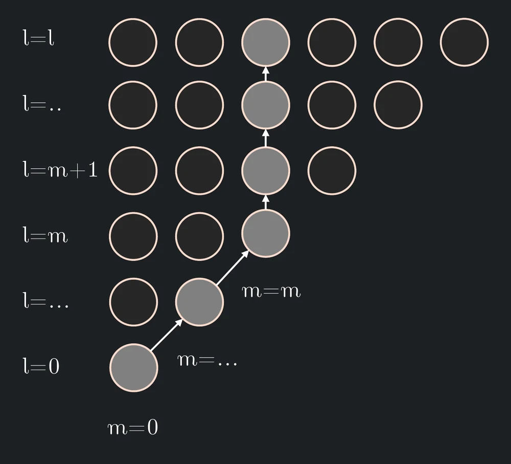
A triangle of circles, with the degree l going up and the order m going across. The path starts at l = 0, m = 0, climbs the diagonal to l = m, m = m, and then goes straight up the column m to the target degree l. — The path to the target. The diagonal builds ${Y'}^m_m$ one factor at a time, then one step gives ${Y'}^m_{m+1}$ and the three-term recurrence climbs the column $m$ up to $\ell$ .

Start from ${Y'}^0_0 = 1$ and walk up the diagonal, multiplying in one factor for each $k = 1 \dots m$ :
${Y'}^k_k = {Y'}^{k-1}_{k-1} \cdot \left(-\sqrt{1 - z^2}\right) \sqrt{\frac{2k + 1}{2k}} \qquad \Bigl(\text{so } {Y'}^m_m = \prod_{k=1}^{m} (-1)\sqrt{1 - z^2}\,\sqrt{\tfrac{2k+1}{2k}}\Bigr)$
One factor at a time keeps the running value in range, where a power of the sine and a product of square roots would underflow.
The first step up the column:
${Y'}^m_{m+1} = z \sqrt{2m + 3} \; {Y'}^m_m$
Then, up to the chosen $\ell$ :
${Y'}^m_{\ell+1} = \sqrt{\frac{(2\ell + 3)(2\ell + 1)}{(\ell + m + 1)(\ell - m + 1)}} \left[ z \, {Y'}^m_\ell - \sqrt{\frac{(\ell + m)(\ell - m)}{(2\ell - 1)(2\ell + 1)}} \; {Y'}^m_{\ell-1} \right]$

The real part is then $\operatorname{Re} Y^m_\ell = {Y'}^m_\ell \cos(m\varphi)/\sqrt{4\pi}$ and the imaginary part $\operatorname{Im} Y^m_\ell = {Y'}^m_\ell \sin(m\varphi)/\sqrt{4\pi}$ . For $m < 0$ the same is done for $|m|$ , and the symmetry gives the result:

Y^{-m}_\ell = (-1)^m \, \overline{Y^m_\ell}

The code is checked against the closed forms for $\ell \le 3$ and against orthonormality: summed over the pixels, the harmonics are orthogonal to each other and each has unit norm.

04 Things to try

Set $m = \pm\ell$ to get the sectoral harmonics, which hug the equator, and $m = 0$ to get the zonal ones, which are bands of latitude. Switch to the imaginary part to see the same pattern turned by a quarter of a wave around the pole. Try a negative $m$ : the pattern keeps its shape and only its sign and phase change. Turn on the grid guide in Tools to read the latitude and longitude. In the Mollweide view the whole sphere is flat and the nodal lines are easy to count. Longitude increases to the left, as on the sky.